Radiometer equation and detectability
Before introducing the radiometer equation in detail, it is helpful to consider the nature of radio sources themselves. On the previous page, you have seen that different continuum sources in radio astronomy exhibit very different radio brightnesses, i.e. flux densities. However, the majority of radio sources are intrinsically very weak.
This naturally leads to an important question:
Can such weak sources be detected with a small radio telescope at all?
To estimate this, we turn to one of the most fundamental tools in radio astronomy — the radiometer equation. It provides a quantitative framework for determining whether a given source can be detected with a specific instrument and observational setup.
A Fundamental Law of Radio Astronomy
The radiometer equation can be regarded as a kind of fundamental law of radio astronomy. It describes how well a weak radio signal can be measured in the presence of noise. In essence, it tells us how the sensitivity of a radio observation depends on both the properties of the instrument and the parameters of the measurement.
In its basic form, the radiometer equation is written as:
\[ \Delta T = \frac{T_{\text{sys}}}{\sqrt{B \tau}} \]
This equation expresses the uncertainty (noise) in a measurement of temperature. The smaller \(\Delta T\), the better a weak signal can be detected.
From Noise Temperature to Source Detection
To relate this to an astronomical source, we connect the measured temperature change \(\Delta T\) to the flux density \(S\) of the source. This is done via the effective collecting area of the antenna.
The effective area of a dish antenna is:
\[ A_{\text{eff}} = \eta \cdot \frac{\pi D^2}{4} \]
where
- \(\eta\) is the aperture efficiency
- \(D\) is the dish diameter
The relation between flux density \(S\) and antenna temperature \(T_A\) is:
\[ T_A = \frac{A_{\text{eff}} \cdot S}{2k} \]
Substituting \(A_{\text{eff}}\) into this equation gives:
\[ T_A = \frac{\eta \cdot \pi D^2 \cdot S}{8k} \]
Combining this with the radiometer equation leads to:
\[ \Delta T = \left( \frac{\eta \cdot D^2 \cdot S}{8k \cdot T_{\text{sys}}} \right) \cdot \sqrt{B \tau} \]
This extended form directly links the detectability of a radio source to physical and observational parameters.
Explanation of Key Parameters
System Temperature \(T_{\text{sys}}\)
The system temperature represents the total noise of the receiving system in Kelvin. It consists of:
- Receiver noise
- Sky noise (Galaxy, atmosphere)
- Ground radiation, spillover, and losses
Typical values:
- Professional radio telescopes: 20–50 K
- Amateur setups (satellite dish + LNB): 100–300 K
Bandwidth \(B\)
The bandwidth is the effective measurement bandwidth in Hz.
- Larger bandwidth → more noise power → better statistical averaging
Typical values:
- Continuum observations: MHz up to ~100 MHz
- Spectral line observations (e.g. HI): kHz to a few MHz
Integration Time \(\tau\)
The integration time is the measurement duration in seconds.
- Longer integration → lower noise
- Improvement follows a square-root law, not linear
What Determines Detectability?
From the extended radiometer equation, the detectability of a source depends on:
- The source’s radio brightness \(S\)
- The antenna aperture \(\eta D^2\)
- The square root of bandwidth and integration time \(\sqrt{B \tau}\)
- The intrinsic noise of the receiving system \(1/T_{\text{sys}}\)
(The Boltzmann constant \(k\) is a physical constant and does not change.)
Physical Interpretation
The radiometer equation predicts:
- A higher source brightness, a larger antenna aperture, or a lower system temperature results in a greater signal rise above the noise floor.
- A longer integration time or a wider bandwidth reduces the noise.
Importantly, the absolute difference between the noise floor and the source signal does not change with increased bandwidth or integration time. However, as the noise decreases, this difference becomes more apparent.
Illustration: Detecting a Weak Source through Averaging
The following figures illustrate how a longer integration time or a larger bandwidth increases the ability to detect a weak continuum source that is hidden within the noise.
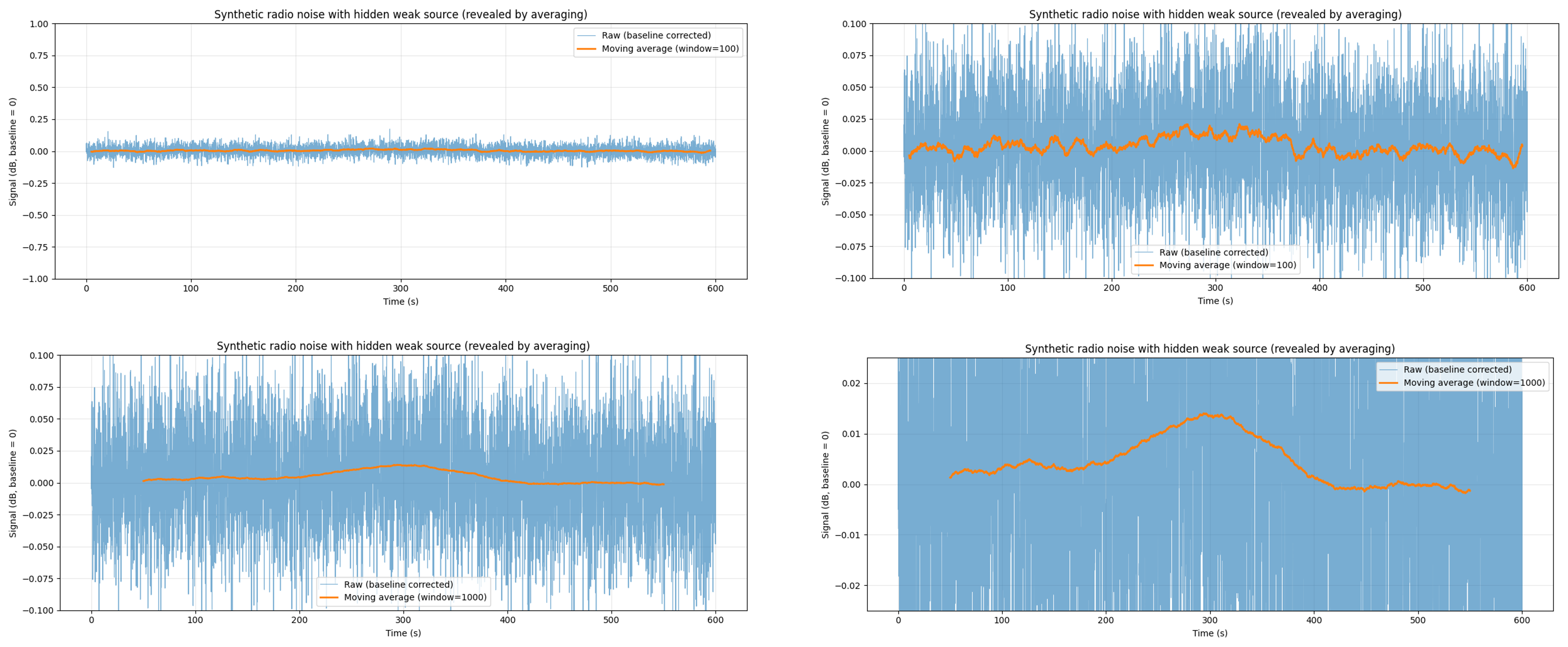
Top left: The raw signal (blue) is shown together with a moving average (window = 100). The signal is dominated by noise, and the hidden source is not yet clearly visible.
Top right: A zoom into the noise. The source is still barely distinguishable.
Bottom left: The moving average is now increased to a window of 1000. The orange curve begins to reveal the presence of a weak underlying signal.
Bottom right: A zoom into the detected source. The source is now clearly visible. The dynamic range of the diagram has been limited to ±0.02 dB to enhance visibility.
These figures demonstrate a key implication of the radiometer equation:
A longer integration time (or equivalently, a larger effective bandwidth) does not increase the absolute signal level, but it reduces the noise, making weak signals progressively more visible.
Bandwidth: A Key Difference
A crucial distinction must be made:
- In radio communication (artificial narrowband transmitters) and in radio-astronomical spectral line observations (e.g. neutral hydrogen, molecular transitions, masers), a smaller bandwidth can improve the signal-to-noise ratio (SNR).
- In continuum radio astronomy, the opposite is true: a larger bandwidth improves the SNR.
Practical Limits in Amateur Radio Astronomy
In amateur radio astronomy:
- Antenna size is limited by cost and space
- System temperature can only be optimized to a certain extent
- Integration time cannot be increased indefinitely
What remains is the bandwidth, which can still be increased effectively.
The Role of the “Second Receiver”
This is where the concept of the Second Receiver, an easy to build broadband detector, becomes particularly important.
Conventional SDR systems typically provide only small bandwidths, usually a few MHz at most. SDR systems with larger bandwidths are expensive and also require high-performance and costly computer hardware.
The Second Receiver operates with very simple hardware:
- It can be used with computers that are more than 20 years old
- It can be assembled from low-cost, widely available components
- It enables very large effective bandwidths of several hundred MHz
This makes it especially suitable for continuum radio astronomy observations, where maximizing bandwidth is the most effective way to improve sensitivity.
With a few simple experiments that you can carry out yourself using basic equipment, you can verify the predictions of the radiometric equation